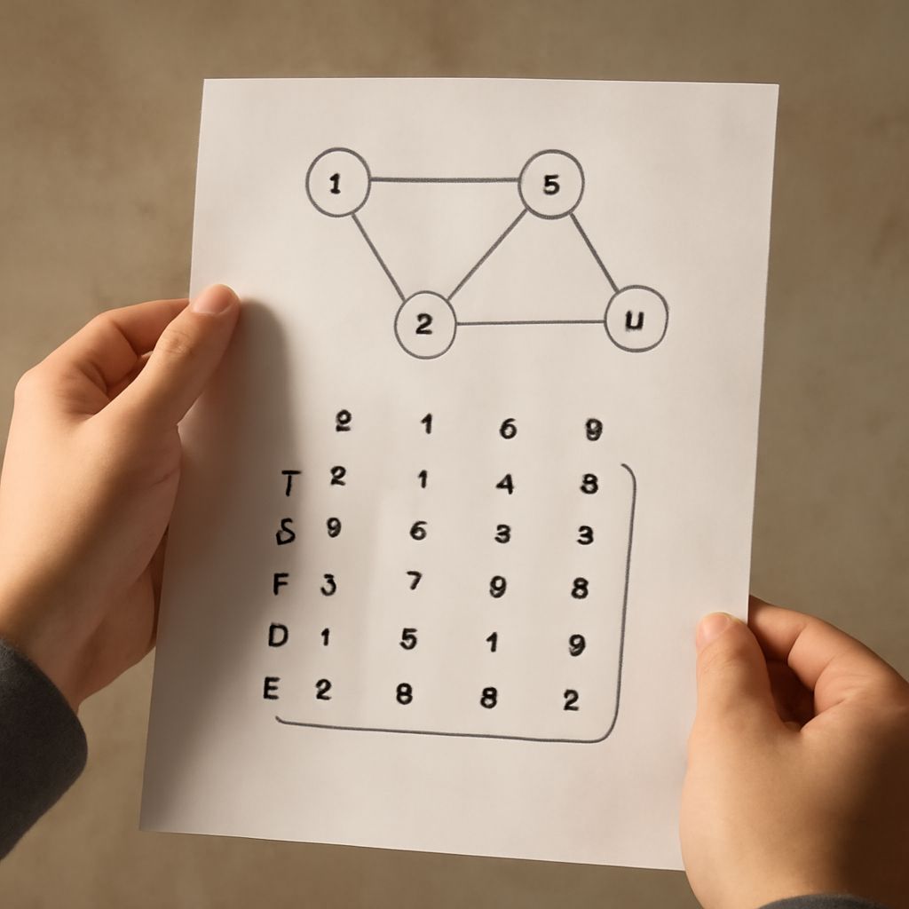
A graph adjacency matrix is a V×V array that records which vertices connect. Choose an order for the vertices, then use that same order for the rows and columns. If the order is A, B, C, D, row A and column A both refer to vertex A, so cell M[A,C] describes the edge between A and C.
An adjacency matrix for a graph works especially well when fast edge checks matter or when the graph is dense. Its meaning changes slightly for undirected, directed, and weighted graphs, but the fixed vertex order remains the foundation.
How an Adjacency Matrix for a Graph Stores Edges
In a simple unweighted graph, a 1 usually means an edge exists and a 0 means no edge exists. Each edge maps to a specific row-column intersection. For example, M[B,D] describes the relationship from B to D; it is separate from M[D,B] when direction matters.
The diagonal cells represent self-loops: M[A,A] concerns an edge from A back to A. If self-loops are not allowed, those cells remain zero or use the representation’s chosen “absent” marker.
Build a Graph Adjacency Matrix from an Undirected Graph
Start with four vertices in this order: A, B, C, D. Suppose the undirected edges are A–B, A–D, B–C, and C–D. Place a 1 at both endpoints’ intersections for every edge:
- Row A: 0 1 0 1
- Row B: 1 0 1 0
- Row C: 0 1 0 1
- Row D: 1 0 1 0
The first value in every row belongs to column A, the second to B, the third to C, and the fourth to D. Because an undirected edge has no preferred direction, M[A,B] and M[B,A] contain the same value. The entire matrix is therefore symmetric across its main diagonal. Changing the vertex order changes the layout, but not the graph’s connections.
How Direction and Weights Change the Same Matrix
Keep the order A, B, C, D, but direct the connections as A→B, A→D, C→B, and D→C. Now each row is the source vertex and each column is the destination:
- Row A: 0 1 0 1
- Row B: 0 0 0 0
- Row C: 0 1 0 0
- Row D: 0 0 1 0
This matrix is asymmetric. For example, M[A,B] is 1, while M[B,A] is 0 because the reverse edge does not exist. To add weights, replace each 1 with the edge’s value. Using weights 5, 2, 4, and 7 for those four directed edges gives rows 0 5 0 2; — 0 — —; — 4 0 —; and — — 7 0. Here, an em dash marks no edge, while 0 on the diagonal means no self-loop.
Do not automatically use zero to mean “no edge” when zero-weight edges are valid. Use a separate presence marker, a null value, or another documented sentinel instead. This distinction prevents a real zero-weight connection from being mistaken for a missing edge.
When Is a Graph Matrix Better Than an Adjacency List?
A graph matrix uses O(V²) storage, regardless of how many edges exist. In return, checking whether an edge connects u and v takes constant time: read M[u,v]. Adding or removing an edge also takes O(1) time when the matrix is already allocated. Scanning all neighbors of one vertex takes O(V), because the algorithm may inspect the whole row.
An adjacency list stores only existing edges, using O(V + E) space, and is usually better for sparse graphs. Neighbor traversal takes O(V + E) across the graph, while checking one edge typically takes O(degree(u)) unless each list uses an additional lookup structure. Choose a graph matrix for dense graphs, repeated direct edge lookups, or algorithms that examine most vertex pairs; choose an adjacency list for sparse graphs and traversal-heavy workloads.