JavaScript data structures are easiest to choose when the required access pattern comes first. Use an array for indexed order, an object for simple string-keyed records, Map for flexible keyed lookup, and Set for uniqueness.

These data structures in JavaScript also support stack and queue patterns. The best data structures JavaScript developers choose depend on whether code needs stable order, repeated values, fast membership checks, or removal from one end.

When are arrays or objects the right choice?

An array is an ordered, index-based collection. It allows duplicates and makes positional reads and updates straightforward, while searching for a value requires scanning. Use it for records displayed in sequence, batches, or data whose position matters.

const colors = [“red”, “blue”, “red”]; The expression colors[1] returns “blue”, and colors.includes(“red”) checks for a value.

A plain object is a record of properties identified by string or symbol keys. It suits fixed fields, configuration, and simple dictionaries. Numeric-looking keys are converted to strings, and inherited properties mean property checks should be deliberate.

const user = { name: “Ari”, role: “editor” }; The expression user.role reads a known property directly.

When should you use Map or Set instead of objects or arrays?

Use Map when a collection is fundamentally a key-value lookup and keys may be any JavaScript value, including objects and functions. Map provides dedicated methods such as set, get, has, and delete, plus a size property.

const prices = new Map([[“book”, 12]]); The expression prices.get(“book”) returns 12.

Use Set when each value should occur only once. It provides membership checks and deletion by value, and it preserves insertion order during iteration, but it does not provide numeric indexes.

const tags = new Set([“js”, “web”, “js”]); The set contains only “js” and “web”; tags.has(“web”) checks membership.

Compare an object with Map by key rules, order, and operations. An object accepts string and symbol property keys and is record-oriented. Map accepts arbitrary key types, has collection-specific operations, and guarantees insertion-order iteration. Object enumeration follows property-key ordering rules, including special handling for integer-like keys, so the two structures are not interchangeable.

Compare an array with Set by the same criteria. An array preserves duplicates, supports indexes, and can represent repeated events in sequence. Set enforces uniqueness and offers direct value membership, making it better for selected IDs, permissions, or visited nodes.

How do stack and queue patterns work with arrays?

A stack uses last-in, first-out access: the newest item is removed first. Arrays implement this pattern efficiently with push and pop.

const stack = []; Then use stack.push(“draft”) to add an item and stack.pop() to remove the newest item.

A queue uses first-in, first-out access: the oldest item is removed first. The simple array pattern adds with push and removes with shift.

const queue = [“first”, “second”]; Use queue.push(“third”), then queue.shift() to remove “first”.

Front removal with shift() can cost O(n) because remaining elements are reindexed. For a growing queue, keep a head index instead: const item = queue[head++]; This avoids repeatedly shifting every remaining element.

How do JavaScript data structures compare by lookup, order, and uniqueness?

• Keyed lookup: choose an object for simple string-keyed records, or Map for arbitrary key types and explicit map operations.
• Order: choose an array for indexed positions, or Set when insertion order matters but duplicates must disappear.
• Uniqueness: choose Set for automatic deduplication; arrays and objects require separate checks or transformation logic.
• Removal pattern: use pop for a stack, shift for a small queue, or a head index for a queue with frequent front removals.

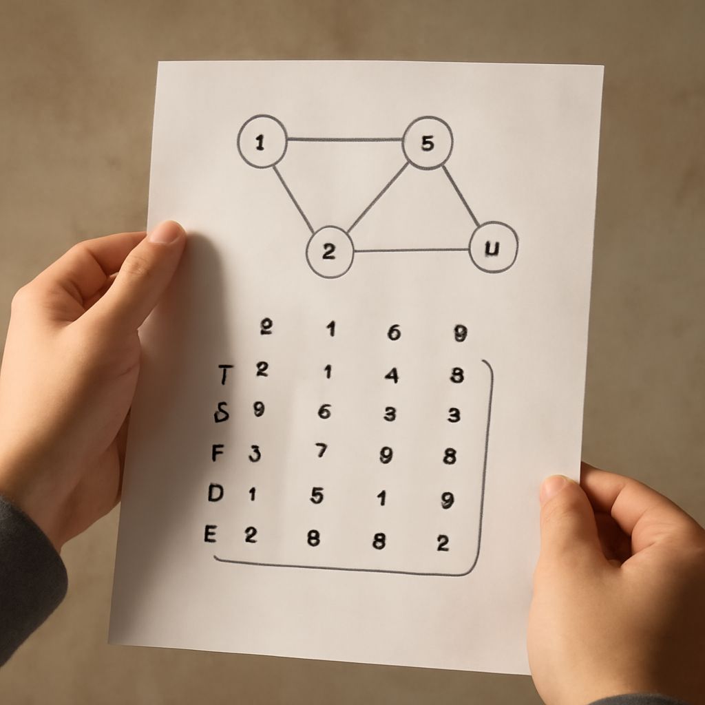
A graph adjacency matrix is a V×V array that records which vertices connect. Choose an order for the vertices, then use that same order for the rows and columns. If the order is A, B, C, D, row A and column A both refer to vertex A, so cell M[A,C] describes the edge between A and C.

An adjacency matrix for a graph works especially well when fast edge checks matter or when the graph is dense. Its meaning changes slightly for undirected, directed, and weighted graphs, but the fixed vertex order remains the foundation.

How an Adjacency Matrix for a Graph Stores Edges

In a simple unweighted graph, a 1 usually means an edge exists and a 0 means no edge exists. Each edge maps to a specific row-column intersection. For example, M[B,D] describes the relationship from B to D; it is separate from M[D,B] when direction matters.

The diagonal cells represent self-loops: M[A,A] concerns an edge from A back to A. If self-loops are not allowed, those cells remain zero or use the representation’s chosen “absent” marker.

Build a Graph Adjacency Matrix from an Undirected Graph

Start with four vertices in this order: A, B, C, D. Suppose the undirected edges are A–B, A–D, B–C, and C–D. Place a 1 at both endpoints’ intersections for every edge:

• Row A: 0 1 0 1
• Row B: 1 0 1 0
• Row C: 0 1 0 1
• Row D: 1 0 1 0

The first value in every row belongs to column A, the second to B, the third to C, and the fourth to D. Because an undirected edge has no preferred direction, M[A,B] and M[B,A] contain the same value. The entire matrix is therefore symmetric across its main diagonal. Changing the vertex order changes the layout, but not the graph’s connections.

How Direction and Weights Change the Same Matrix

Keep the order A, B, C, D, but direct the connections as A→B, A→D, C→B, and D→C. Now each row is the source vertex and each column is the destination:

• Row A: 0 1 0 1
• Row B: 0 0 0 0
• Row C: 0 1 0 0
• Row D: 0 0 1 0

This matrix is asymmetric. For example, M[A,B] is 1, while M[B,A] is 0 because the reverse edge does not exist. To add weights, replace each 1 with the edge’s value. Using weights 5, 2, 4, and 7 for those four directed edges gives rows 0 5 0 2; — 0 — —; — 4 0 —; and — — 7 0. Here, an em dash marks no edge, while 0 on the diagonal means no self-loop.

Do not automatically use zero to mean “no edge” when zero-weight edges are valid. Use a separate presence marker, a null value, or another documented sentinel instead. This distinction prevents a real zero-weight connection from being mistaken for a missing edge.

When Is a Graph Matrix Better Than an Adjacency List?

A graph matrix uses O(V²) storage, regardless of how many edges exist. In return, checking whether an edge connects u and v takes constant time: read M[u,v]. Adding or removing an edge also takes O(1) time when the matrix is already allocated. Scanning all neighbors of one vertex takes O(V), because the algorithm may inspect the whole row.

An adjacency list stores only existing edges, using O(V + E) space, and is usually better for sparse graphs. Neighbor traversal takes O(V + E) across the graph, while checking one edge typically takes O(degree(u)) unless each list uses an additional lookup structure. Choose a graph matrix for dense graphs, repeated direct edge lookups, or algorithms that examine most vertex pairs; choose an adjacency list for sparse graphs and traversal-heavy workloads.

The union-find algorithm maintains a changing collection of non-overlapping sets. Its core operations are make-set, which creates a singleton set; find, which returns a set’s representative; and union, which merges two sets. It supports connectivity tests without storing every member relationship explicitly.

The same technique, called disjoint set union, represents each set with a parent forest. The implementation below starts with that forest, then adds path compression and union by rank so repeated operations stay near-constant in amortized time.

How does the union-find algorithm represent sets?

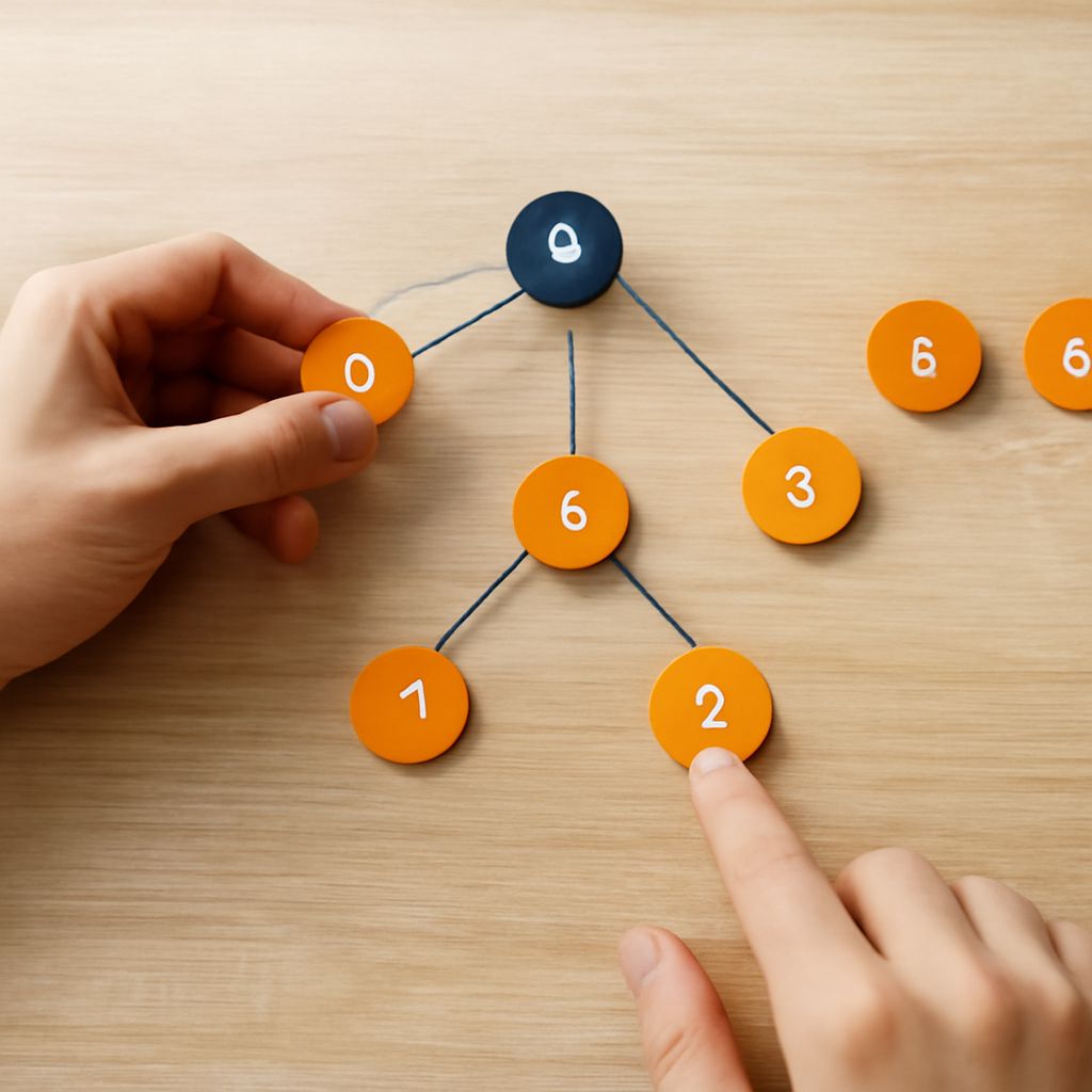
A set is a component: a group of elements connected through previous union operations. Each element is a node with one parent pointer. A root points to itself, so parent[x] = x identifies the root. That root is the component’s representative.

make-set(x) creates a new component containing only x. It sets parent[x] = x and initializes a rank or size value. Initially, every item is its own representative. When two components merge, one root becomes a child of the other root. The resulting parent forest encodes membership: following parent links eventually reaches the representative.

To test whether two elements belong to the same component, compare their representatives. If find(a) = find(b), they are connected according to the unions performed so far. This structure tracks connectivity efficiently; it is not intended to enumerate the full route between two vertices.

How do you implement a union-find data structure with make-set, find, and union?

Store parent and rank in arrays or maps. The following pseudocode includes both standard optimizations:

make-set(x): Set parent[x] = x and rank[x] = 0.

find(x): If parent[x] is not x, replace parent[x] with find(parent[x]). Return parent[x].

union(a, b): Compute rootA = find(a) and rootB = find(b). If the roots match, stop. Otherwise, attach the lower-rank root below the higher-rank root. If the ranks match, choose either root as the parent and increase its rank by one.

For elements A through E, initialization produces:

• Initial: parent = {A:A, B:B, C:C, D:D, E:E}; rank = {A:0, B:0, C:0, D:0, E:0}.
• union(A, B): attach B to A; parent[B] = A and rank[A] = 1.
• union(C, D): attach D to C; parent[D] = C and rank[C] = 1.
• union(A, C): both roots have rank 1, so attach C to A and raise rank[A] = 2. D still points to C.
• union(D, E): finding D reaches A through C, then compresses D to point directly to A. E attaches to A.

The final parent array is {A:A, B:A, C:A, D:A, E:A}, with A as representative and rank A equal to 2. Calling find(D) now returns A immediately.

How do path compression and union by rank work?

Path compression changes every node visited by find to point directly to the root. In the example, D initially points to C, and C points to A. After find(D), D points to A. The operation may traverse several links once, but later searches from D skip those intermediate nodes.

Union by rank controls how roots are linked. Rank estimates a tree’s height: attach the smaller-rank tree beneath the larger-rank tree, and increase rank only when equal ranks merge. This avoids creating long chains. A size array can replace rank by attaching the smaller component to the larger one.

How does disjoint set union achieve near-constant amortized time?

Without either optimization, repeated unions can form a chain, making find take O(n) time. Union by rank limits tree height to O(log n), while path compression flattens the portions of trees that searches actually visit. Used together, a sequence of m operations on n elements takes O(m α(n)) amortized time, where α is the inverse Ackermann function and grows so slowly that it is effectively constant for practical input sizes. Each make-set is O(1), and the arrays require O(n) space.

The AVL tree balance factor shows whether a node’s left and right subtrees remain close in height. After each insertion, calculate this value while moving from the new node toward the root. A value outside the range -1 to 1 identifies the ancestor that needs a rotation.

These AVL tree examples use one height convention and one sign convention throughout, so each LL, RR, LR, or RL case follows directly from the observed values.

What Is the AVL Tree Balance Factor? Set Height and Sign Convention First

Set the height of an empty child to 0 and the height of a leaf to 1. For every node:

height(node) = 1 + max(height(left), height(right))

Using left height minus right height, the balance factor formula is:

balance factor = height(left subtree) − height(right subtree)

• +1: the left subtree is one level taller.
• 0: both subtrees have equal height.
• -1: the right subtree is one level taller.

An AVL node is height-balanced when its factor is -1, 0, or +1. A factor of +2 means left-heavy imbalance; -2 means right-heavy imbalance. The sign convention matters: reversing the subtraction would reverse the case labels.

How Do You Calculate the Balance Factor in an AVL Tree and Find the First Unbalanced Ancestor?

After inserting a key as in an ordinary binary search tree, start at that new leaf and move upward. At each node, update its height first, then calculate its balance factor. The first unbalanced ancestor is the first node encountered with a factor of +2 or -2. Because the search proceeds upward, this is the lowest unbalanced ancestor and normally the point where you apply the rotation.

1. Insert the key according to binary-search-tree ordering.
2. Recompute each ancestor’s height using the larger child height.
3. Calculate left height minus right height.
4. Use the heavy child and the inserted key’s direction to identify LL, RR, LR, or RL.
5. Rotate, then recompute heights from the lowest changed node upward.

Which AVL Tree Examples Show LL and RR Rotations With Updated Heights?

LL case: Insert 30, then 20, then 10. The path leans left twice:

30(+2)
↙ 20(+1)
↙ 10(0)

Node 30 is the first unbalanced ancestor. Apply one right rotation at 30. Node 20 becomes the root, with 10 as its left child and 30 as its right child. Each leaf has height 1; node 20 has height 2 and balance factor 0. The rotation changes structure first, so calculate the lower node’s height before the new root’s height.

RR case: Insert 10, then 20, then 30. The path leans right twice. Node 10 has factor -2, so apply one left rotation at 10. Node 20 becomes the root, with 10 on the left and 30 on the right. Both leaves have height 1, and node 20 has height 2 with factor 0.

How Does AVL Tree Balancing Resolve LR and RL Cases With Updated Heights?

LR case: Insert 30, then 10, then 20. Node 30 has factor +2, but its left child, 10, has factor -1. This is a left-right bend, so use two rotations:

1. Rotate left at 10. The subtree becomes 20 with 10 as its left child.
2. Rotate right at 30. Node 20 becomes the subtree root, with 10 and 30 as children.

After the structural changes, 10 and 30 each have height 1. Node 20 receives height 2 and factor 0.

RL case: Insert 10, then 30, then 20. Node 10 has factor -2, while its right child, 30, has factor +1. Apply the mirror sequence:

1. Rotate right at 30, making 20 the root of that subtree with 30 on the right.
2. Rotate left at 10, making 20 the subtree root with 10 on the left.

Again, the two leaves have height 1, and the new subtree root 20 has height 2 and factor 0. This is the practical rule for AVL tree balancing: single-direction growth uses one rotation; a bend uses the child rotation first, followed by the opposite rotation at the unbalanced ancestor.

Stack vs queue comes down to the required access pattern. A stack uses LIFO (last in, first out), so the newest item leaves first. A queue uses FIFO (first in, first out), so the oldest item leaves first. Choose a stack for nested work, undo behavior, or backtracking; choose a queue for arrival-order processing and fair turn-taking.

The difference between stack and queue behavior becomes clear when both structures receive the same items. Their operation names, implementations, and use cases follow from that ordering rule.

Stack vs queue: LIFO or FIFO, and what order do items leave?

Insert the items A, B, and C in that order.

• Stack: A is placed first, then B, then C. Removing items returns C, B, and A.
• Queue: A is placed first, then B, then C. Removing items returns A, B, and C.

In a stack, the insertion and removal point is the top. Each new item covers the previous one, like a pile of plates. The most recently added item is therefore immediately available.

In a queue, insertion occurs at the rear and removal occurs at the front. Items remain in their arrival order, like people waiting in a line. A standard queue removes the oldest waiting item rather than the newest one.

Queue vs stack: How do their operations differ?

Stack operations focus on one accessible end:

• Push: adds an item to the top.
• Pop: removes and returns the top item.
• Peek or top: reads the top item without removing it.

Queue operations separate the entry and exit ends:

• Enqueue: adds an item at the rear.
• Dequeue: removes and returns the item at the front.
• Front or peek: reads the next item without removing it.

With a suitable implementation, push, pop, enqueue, dequeue, and peek are expected O(1) operations. That means the operation takes constant time on average or by design, regardless of how many items are stored. A queue implemented by repeatedly removing index zero from a basic array can become O(n), because every remaining item may need to shift. A circular buffer or linked queue avoids that cost.

What is the difference between stack and queue implementations?

An array or dynamic array is a natural stack implementation. Adding and removing at the array’s end usually takes O(1) amortized time, while accessing the top is direct. A linked-list stack can also provide O(1) push and pop when the head represents the top. It uses extra memory for links but does not require contiguous storage.

Queues are commonly implemented with a circular array, a linked list, or a double-ended queue (deque). A circular array keeps front and rear positions moving through a fixed or resizable buffer, so it does not shift every remaining item after dequeue. A linked queue maintains references to both the front and rear nodes, providing O(1) enqueue and dequeue.

Both structures typically use O(n) space for n items. The practical choice depends on memory layout, resizing behavior, concurrency requirements, and whether the program needs access at one end or two. Neither structure normally supports efficient arbitrary-position removal; that requirement may call for a different data structure.

When should you use stacks and queues?

Use stacks for problems where the latest unfinished task must be handled first:

• Function calls and recursion: call frames form a stack, with the newest active call completed first.
• Parsing nested syntax: parentheses, brackets, and HTML-like tags can be matched against recently opened elements.
• Undo and redo: actions are stored so the most recent change can be reversed first.
• Depth-first search and backtracking: the algorithm follows one path, then returns to the latest decision point when that path fails.

Use queues when work should be processed in arrival order:

• Breadth-first search: nodes are visited level by level, with earlier discoveries handled first.
• Task pipelines: jobs wait in sequence for a worker or service to process them.
• Event handling: incoming events can be processed in the order they were received.
• Request scheduling: a basic service queue gives earlier requests an opportunity before later ones.

In short, stacks and queues solve opposite ordering problems: choose the stack’s newest-first behavior for nesting and backtracking, and the queue’s oldest-first behavior for orderly flow through a system.

An adjacency list stores each vertex with its neighboring vertices, rather than placing every possible pair in a grid. It is usually the most efficient representation for a sparse graph, where the number of edges is much smaller than the square of the number of vertices.

An adjacency list is not an ordered path through a graph. Each entry records local connections; a traversal algorithm chooses the next vertex separately.

What is an adjacency list?

An adjacency list maps every vertex to a collection of adjacent vertices. In an adjacency list graph, the outer structure is commonly an array or map, and each value is a dynamic list. An array works well when vertices have numeric indexes. A map is useful when labels such as “A” or “Airport 12” identify vertices.

For a vertex v, its list contains the vertices reachable by one edge from v. The number of entries is its degree in an undirected graph or its out-degree in a directed graph. Isolated vertices still receive an empty list so that the representation includes every vertex.

How do you build a graph adjacency list from edge data?

Start with the vertices, create an empty list for each one, and then process each edge. Consider this undirected edge data:

• A-B
• A-C
• B-D
• C-D

The matching adjacency-list representation is:

• A: B, C
• B: A, D
• C: A, D
• D: B, C

Each undirected edge appears twice. The edge A-B is recorded in A’s list and B’s list, allowing neighbor lookup from either endpoint. A simple construction procedure is:

1. Initialize an empty list for every vertex.
2. For an edge between u and v, append v to u’s list.
3. Because the edge is undirected, append u to v’s list as well.

If the input can contain parallel edges, append each occurrence unless the application requires duplicate removal. A set can enforce unique neighbors, but it changes the storage structure and may add overhead.

How does an adjacency list represent directed and weighted edges?

Direction determines which list receives an edge. For directed edges A→B, A→C, and C→B, the list is:

• A: B, C
• B: empty
• C: B

The reverse connection is not implied. If an algorithm must find incoming neighbors, it can maintain a second reverse adjacency list or scan all lists.

Weighted edges store a neighbor together with its weight. For example, the weighted edge data A→B with cost 5 and A→C with cost 2 becomes:

• A: (B, 5), (C, 2)
• B: empty
• C: empty

The weight can represent distance, price, capacity, or another application-specific value. Adding weights changes the value stored beside each neighbor, not the basic adjacency-list structure or its usual asymptotic costs.

When is an adjacency list for a graph better than an adjacency matrix?

For V vertices and E edges, an adjacency list uses O(V + E) space when each edge is stored once in a directed graph or twice in an undirected graph. This is efficient for sparse graphs because it stores actual connections instead of all possible connections.

• Iterating neighbors: O(degree(v)) for vertex v. The algorithm visits only listed neighbors.
• Testing a specific edge: usually O(degree(v)) when scanning the list for the target. A hash-based neighbor set provides O(1) average lookup, with additional memory overhead.
• Adding an edge: commonly O(1) when appending to a list, unless duplicate checking is required.

An adjacency matrix uses O(V²) space and provides O(1) edge testing by checking one cell. However, finding all neighbors of a vertex requires scanning its entire row, which costs O(V), including cells for absent edges. Choose an adjacency list when neighbor traversal and compact storage matter, especially for sparse networks. Choose a matrix when the graph is dense or constant-time edge tests are more important than memory use.