An XOR truth table shows the output of an exclusive OR gate for every possible input combination. The output is true, or 1, when exactly one input is true, or 1. It is false, or 0, when both inputs match: both are 0 or both are 1.

For two inputs named A and B, the rule is “one but not both.” This rule connects directly to the Boolean expression, the circuit symbol, and practical bit comparisons.

What does an XOR truth table show about one input but not both?

An XOR gate has two inputs and one output, commonly written as Y = A ⊕ B. The circled plus sign, ⊕, is the standard Boolean symbol for exclusive OR.

Use these checks to evaluate the output:

• If A is 0 and B is 0, neither input is true, so Y is 0.
• If A is 0 and B is 1, exactly one input is true, so Y is 1.
• If A is 1 and B is 0, exactly one input is true, so Y is 1.
• If A is 1 and B is 1, both inputs are true, so Y is 0.

The last case distinguishes XOR from inclusive OR. An inclusive OR gate produces 1 when both inputs are 1; an XOR gate produces 0 because the inputs are not different.

How does an XOR logic table list all four input pairs?

An XOR logic table lists each possible pair once. With two binary inputs, there are 2², or four, combinations. The output column records whether the inputs differ.

• A = 0, B = 0 → Y = 0: the inputs are equal.
• A = 0, B = 1 → Y = 1: the inputs are different.
• A = 1, B = 0 → Y = 1: the inputs are different.
• A = 1, B = 1 → Y = 0: the inputs are equal.

This makes XOR useful for detecting disagreement. The output is high only for the two mixed rows, 01 and 10. It is low for the matching rows, 00 and 11. Reading the rows in this order prevents the common error of assigning a true output to the 11 case.

What Boolean expressions are equivalent to XOR?

The compact expression is:

Y = A ⊕ B

An equivalent AND-OR-NOT expression expands the one-but-not-both rule into two valid paths:

Y = (A AND NOT B) OR (NOT A AND B)

The first term is true when A is 1 and B is 0. The second term is true when A is 0 and B is 1. Since either term can produce the output, the two terms are joined with OR.

In common Boolean algebra notation, the same expression is written:

Y = A′B + AB′

Here, the apostrophe means NOT, adjacent variables mean AND, and the plus sign means OR. Some programming and digital-logic contexts use the caret, ^, for XOR, especially in bitwise operations. The surrounding language or circuit notation determines whether that symbol means XOR.

How do you recognize an XOR gate diagram?

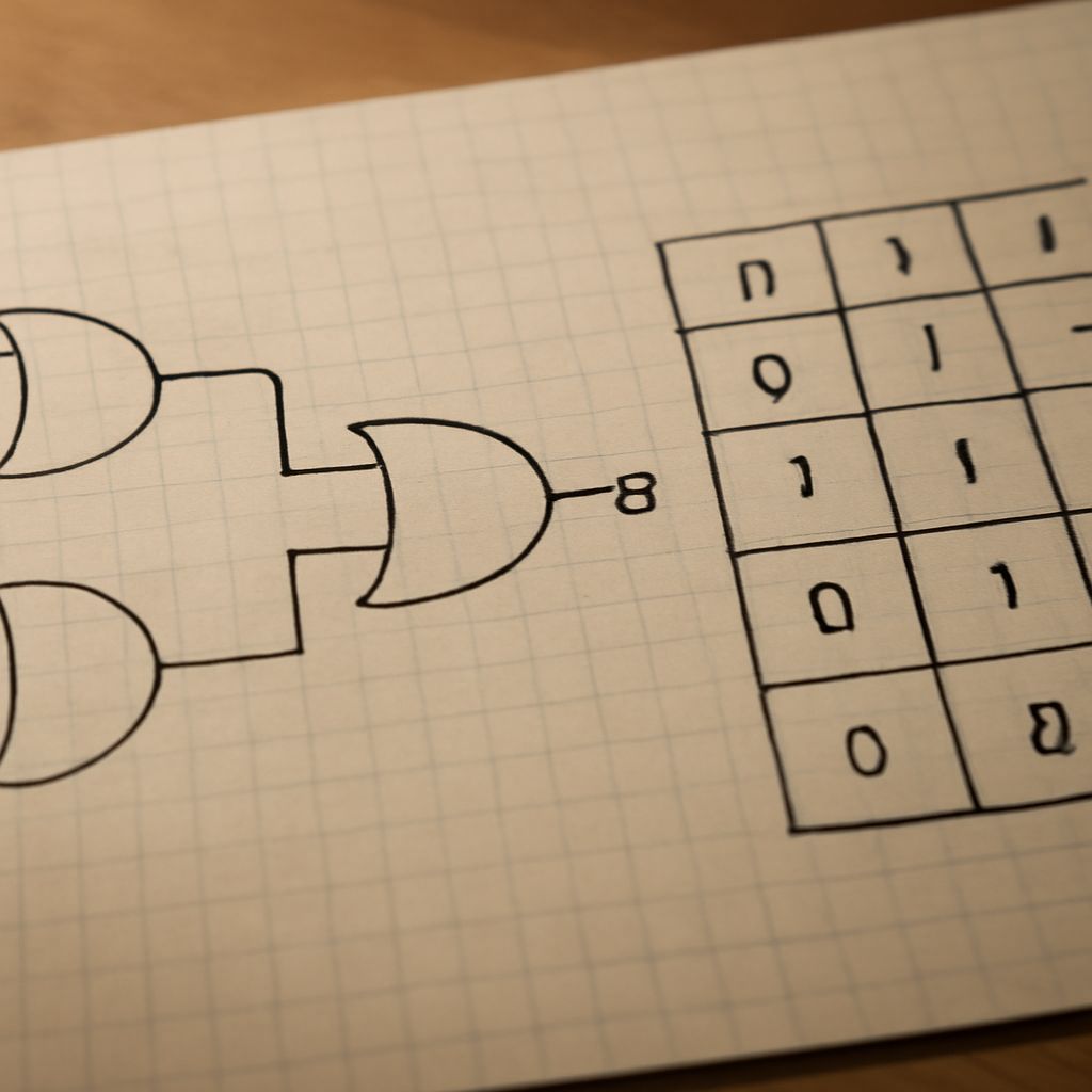
An XOR gate diagram uses the familiar curved outline of an OR gate, with one important addition: a second curved line appears on the input side, in front of the main gate outline. That extra curve identifies the exclusive function.

A labeled two-input diagram can be read like this:

A (input 1) + B (input 2) → XOR gate → Y (output)

• A and B: the two incoming binary signals.
• ⊕: the XOR operation between those signals.
• Y: the output, equal to 1 only when A and B differ.

For example, compare the bit strings 1011 and 1001 position by position with XOR:

1011 ⊕ 1001 = 0010

The 1 in the result marks the position where the input bits differ. Matching bit pairs produce 0, while differing pairs produce 1. The same behavior can toggle a control bit: XOR with 1 changes a bit, while XOR with 0 leaves it unchanged.

Truth tables for logic gates show every possible input combination and the resulting output. For a two-input gate, inputs are usually labeled A and B, while the output is Y. A 0 represents false or low, and a 1 represents true or high.

Read each row from left to right: identify the input values, apply the gate’s Boolean rule, and then check the output column. The complete set of rows makes gate truth tables useful for predicting circuit behavior without inspecting the circuit’s internal design.

How do you read truth tables for logic gates?

A two-input truth table has four rows because two binary inputs produce four combinations: 00, 01, 10, and 11. The order of A and B matters when reading a row, even though several basic gates produce the same result when the inputs are swapped.

• A = 0, B = 0: both inputs are low.
• A = 0, B = 1: A is low and B is high.
• A = 1, B = 0: A is high and B is low.
• A = 1, B = 1: both inputs are high.

The expression beside a gate states its Boolean operation. For example, Y = A · B means “A AND B.” The output column translates that operation into a result for each row.

What does a truth table for an AND gate show?

An AND gate uses the expression Y = A · B. Its plain-language rule is: the output is 1 only when both inputs are 1. Any 0 input makes the output 0.

• A = 0, B = 0 → Y = 0
• A = 0, B = 1 → Y = 0
• A = 1, B = 0 → Y = 0
• A = 1, B = 1 → Y = 1

This truth table for an AND gate is the reference for understanding NAND, which reverses the AND output.

How do OR, NOT, NAND, and NOR gate truth tables work?

An OR gate uses Y = A + B. Its rule is: the output is 1 when at least one input is 1, including when both inputs are 1.

• 0, 0 → 0
• 0, 1 → 1
• 1, 0 → 1
• 1, 1 → 1

A NOT gate has one input and uses Y = ¬A. It inverts its input, so 0 becomes 1 and 1 becomes 0.

• A = 0 → Y = 1
• A = 1 → Y = 0

A NAND gate uses Y = ¬(A · B). It is an AND gate followed by NOT, so its output is the inverse of the AND output: it is 0 only when both inputs are 1.

• 0, 0 → 1
• 0, 1 → 1
• 1, 0 → 1
• 1, 1 → 0

A NOR gate uses Y = ¬(A + B). It is an OR gate followed by NOT, so its output is the inverse of the OR output: it is 1 only when both inputs are 0.

• 0, 0 → 1
• 0, 1 → 0
• 1, 0 → 0
• 1, 1 → 0

How do XOR and XNOR gate truth tables differ?

An XOR gate uses Y = A ⊕ B. Its rule is: the output is 1 when exactly one input is 1. XOR is not the same as inclusive OR because XOR returns 0 when both inputs are true.

• 0, 0 → 0
• 0, 1 → 1
• 1, 0 → 1
• 1, 1 → 0

An XNOR gate uses Y = ¬(A ⊕ B). It is XOR followed by NOT, so it inverts the XOR output. The output is 1 when the inputs match and 0 when they differ.

• 0, 0 → 1
• 0, 1 → 0
• 1, 0 → 0
• 1, 1 → 1

Hexadecimal arithmetic uses the same column method as decimal arithmetic, but each column is based on 16. This guide covers hex subtraction, hexadecimal addition, hex multiplication, hexadecimal subtraction, and hexadecimal multiplication with carries, borrows, and decimal checks.

Align operands by place value, work from right to left, and use the same digit-value map for every operation.

Hex Digits and Place Values in Base 16

Hexadecimal uses 16 symbols. The letters continue the values after 9:

• 0–9: values 0 through 9
• A: 10, B: 11, C: 12
• D: 13, E: 14, F: 15

From right to left, place values are 16⁰, 16¹, 16², and so on. For example, 2A7 equals 2 × 256 + 10 × 16 + 7. Always right-align operands so units, sixteens, and 256s share a column.

Hexadecimal Addition With Carries

In hexadecimal addition, a column produces a carry when its total is 16 or more. Divide the column total by 16: write the remainder in the current column and carry the quotient to the next column. A carry is not made at 10, as it is in base 10.

A complete addition example with a carry

Add 2A7 + 19D:

1. Units: 7 + D = 7 + 13 = 20 decimal, or 14 in hexadecimal. Write 4 and carry 1.
2. Sixteens: A + 9 + 1 = 10 + 9 + 1 = 20 decimal, or 14 hexadecimal. Write 4 and carry 1.
3. 256s: 2 + 1 + 1 = 4. Write 4.

Therefore, 2A7 + 19D = 444. The repeated carries occur because each completed column contains 16 units of the next place value.

Hex Subtraction With Borrows

For hexadecimal subtraction, subtract each right-aligned column from right to left. If the top digit is smaller, borrow 1 from the next column. That borrowed 1 equals 16 units in the current column, not 10.

A hexadecimal subtraction example

Subtract 1C7 from 3A2:

1. Units: 2 is smaller than 7, so borrow 1 from A. The units become 2 + 16 = 18, and 18 − 7 = 11, which is B. The A becomes 9.
2. Sixteens: 9 is smaller than C, so borrow 1 from 3. The column becomes 9 + 16 = 25, and 25 − 12 = 13, which is D. The 3 becomes 2.
3. 256s: 2 − 1 = 1.

The result is 3A2 − 1C7 = 1DB. Each borrow adds 16 to the column being solved, while reducing the next column by 1.

Hexadecimal Multiplication and Decimal Verification

Hexadecimal multiplication follows long multiplication. Multiply by each digit, convert each product into a hexadecimal digit plus carry, shift each partial product one place for every position moved left, and then add the partial products.

A hex multiplication example

Multiply 2F × 1A:

1. Multiply 2F by A. F × A is 15 × 10 = 150 decimal, which is 96 hexadecimal. Write 6 and carry 9. Then 2 × 10 + 9 = 29 decimal, or 1D hexadecimal. This partial product is 1D6.
2. Multiply 2F by 1. The partial product is 2F, shifted one hexadecimal place left because 1 is in the sixteens column: 2F0.
3. Add the partial products: 1D6 + 2F0 = 4C6. In the middle column, D + F = 28 decimal, or 1C hexadecimal; write C and carry 1.

Therefore, 2F × 1A = 4C6.

Verify the result in decimal

Convert the factors and result using powers of 16:

• 2F = 2 × 16 + 15 = 47
• 1A = 1 × 16 + 10 = 26
• 4C6 = 4 × 256 + 12 × 16 + 6 = 1,222

Now check the multiplication: 47 × 26 = 1,222. The decimal product matches 4C6, confirming the hexadecimal result.

This hex to binary table aligns every integer from 0 through 31 with its eight-bit binary and two-digit hexadecimal form. It also works as a quick binary to decimal chart when you need to verify a value.

Use the fixed-width columns for lookup, then apply place-value arithmetic or four-bit grouping when converting values beyond the chart.

Hex to Binary Table: 0–31 Decimal, 8-Bit Binary, and 2-Digit Hex

Each row follows the order decimal — 8-bit binary — 2-digit hexadecimal. Hexadecimal letters use uppercase notation from A through F.

• 0 — 00000000 — 00
• 1 — 00000001 — 01
• 2 — 00000010 — 02
• 3 — 00000011 — 03
• 4 — 00000100 — 04
• 5 — 00000101 — 05
• 6 — 00000110 — 06
• 7 — 00000111 — 07
• 8 — 00001000 — 08
• 9 — 00001001 — 09
• 10 — 00001010 — 0A
• 11 — 00001011 — 0B
• 12 — 00001100 — 0C
• 13 — 00001101 — 0D
• 14 — 00001110 — 0E
• 15 — 00001111 — 0F
• 16 — 00010000 — 10
• 17 — 00010001 — 11
• 18 — 00010010 — 12
• 19 — 00010011 — 13
• 20 — 00010100 — 14
• 21 — 00010101 — 15
• 22 — 00010110 — 16
• 23 — 00010111 — 17
• 24 — 00011000 — 18
• 25 — 00011001 — 19
• 26 — 00011010 — 1A
• 27 — 00011011 — 1B
• 28 — 00011100 — 1C
• 29 — 00011101 — 1D
• 30 — 00011110 — 1E
• 31 — 00011111 — 1F

Read the Fixed-Width Columns in the Binary to Decimal Chart

The decimal column shows the ordinary base-10 value. The binary column always has eight positions, while the hexadecimal column always has two digits. Leading zeros preserve that width without changing the value: decimal 5 is binary 00000101 and hexadecimal 05.

For binary, each position represents a power of two. From right to left, the eight-bit positions are 1, 2, 4, 8, 16, 32, 64, and 128. A 1 means that position contributes to the total; a 0 means it does not.

Hexadecimal uses sixteen symbols: 0 through 9 represent zero through nine, and A through F represent 10 through 15. This makes each hexadecimal digit equivalent to exactly four binary bits.

Use the Binary to Decimal Table for Place Values and a Worked Check

The binary to decimal table can be recreated by adding the place values beneath every 1. Start at the rightmost bit with 1, double each value as you move left, and ignore positions containing 0.

For example, convert 00010111 to decimal:

0 × 128 + 0 × 64 + 0 × 32 + 1 × 16 + 0 × 8 + 1 × 4 + 1 × 2 + 1 × 1 = 16 + 4 + 2 + 1 = 23.

The table confirms the result: decimal 23 is binary 00010111 and hexadecimal 17. The same arithmetic works for any binary length. For a value with more than eight bits, continue the place values to the left with 256, 512, 1,024, and higher powers of two.

Convert Between Bases with the Binary to Hexadecimal Table Using Four-Bit Nibbles

For binary-to-hexadecimal conversion, divide the binary number into four-bit groups called nibbles, starting from the right. If the leftmost group has fewer than four bits, add leading zeros. Convert each nibble independently using the values from 0000 through 1111.

For a value in the chart, convert 00011111:

00011111 → 0001 1111 → 1F.

The first nibble, 0001, equals hexadecimal 1. The second nibble, 1111, equals hexadecimal F. Therefore, binary 00011111 equals hexadecimal 1F and decimal 31.

Reverse the process for hexadecimal-to-binary conversion: replace every hexadecimal digit with its four-bit equivalent and join the groups. For example, hexadecimal D6 is beyond the 0–31 chart:

D6 → 1101 0110 → 11010110.

Thus, D6 equals binary 11010110. Its decimal value is 13 × 16 + 6 = 214. Keep all four bits in each nibble, including zeros, so every hexadecimal digit remains aligned with its binary representation.

Using lowercase text and ASCII-compatible UTF-8, hello in binary is 01101000 01100101 01101100 01101100 01101111 (ASCII-compatible UTF-8, lowercase “hello”). The answer to how to say hello in binary follows the same letter-by-letter process for every character.

In this encoding, each lowercase English letter uses one byte, or eight bits. The spaces shown between groups separate bytes; they are formatting and are not part of the word unless a character space is explicitly encoded.

Hello in binary: What does each byte mean?

For lowercase hello in ASCII-compatible UTF-8, each character has an ASCII-compatible code point, a decimal byte value, and a padded eight-bit binary value:

• h — decimal 104 — 01101000
• e — decimal 101 — 01100101
• l — decimal 108 — 01101100
• l — decimal 108 — 01101100
• o — decimal 111 — 01101111

The repeated l produces the repeated byte. Because these letters are within the ASCII range, their UTF-8 bytes match their ASCII values.

How to say hello in binary, step by step

1. Write the greeting in the intended case: hello, all lowercase.
2. Separate it into characters: h, e, l, l, and o.
3. Convert each character to its decimal ASCII-compatible value.
4. Convert each decimal value to base two and add leading zeroes until every result has eight bits.
5. Join the bytes in their original order.

That process creates the binary for hello: 01101000 01100101 01101100 01101100 01101111 (ASCII-compatible UTF-8, lowercase “hello”). Keeping the eight-bit groups visible makes the result easier to check and decode.

Hi in binary: How does the shorter greeting convert?

For lowercase hi in ASCII-compatible UTF-8, the character mapping is:

• h — decimal 104 — 01101000
• i — decimal 105 — 01101001

Therefore, hi in binary is 01101000 01101001 (ASCII-compatible UTF-8, lowercase “hi”). It contains two eight-bit bytes, one for each letter.

Thank you in binary: How is the space handled?

For lowercase thank you in ASCII-compatible UTF-8, include the space as its own character. Its decimal value is 32, represented by the eight-bit byte 00100000.

• t — decimal 116 — 01110100
• h — decimal 104 — 01101000
• a — decimal 97 — 01100001
• n — decimal 110 — 01101110
• k — decimal 107 — 01101011
• space — decimal 32 — 00100000
• y — decimal 121 — 01111001
• o — decimal 111 — 01101111
• u — decimal 117 — 01110101

So, thank you in binary is 01110100 01101000 01100001 01101110 01101011 00100000 01111001 01101111 01110101 (ASCII-compatible UTF-8, lowercase “thank you,” including the space).

If the bytes are written as one continuous sequence, they become 011101000110100001100001011011100110101100100000011110010110111101110101 (ASCII-compatible UTF-8, lowercase “thank you,” including the space). To decode it, start from the left and regroup the bits into sets of eight. Convert each byte back to its decimal value, then match that value to its character. The byte 00100000 becomes the visible gap between thank and you.

Two’s complement is the standard way to represent signed integers in a fixed number of binary bits. It uses the bit pattern itself to encode positive values, zero, and negative values, allowing the same binary adder to handle signed and unsigned-looking bit patterns.

This explanation uses an eight-bit word throughout. The two’s-complement binary method connects each pattern to a signed value through positional weights, then uses ordinary binary addition for arithmetic.

Why does signed binary need two’s complement?

Bits naturally represent nonnegative values: with eight bits, 00000000 through 11111111 represent 0 through 255 when interpreted as unsigned binary. Signed integers need a way to represent values below zero as well as positive values.

A signed encoding must also support one representation of zero and practical addition and subtraction. Two’s complement meets these needs without storing a separate sign-and-magnitude field. Every bit contributes to the value, including the most significant bit (MSB), whose weight is negative rather than positive.

In binary two’s complement, the MSB signals the value range through its weight, but it is not a detachable sign bit attached to an unchanged magnitude. Changing that bit changes the complete numerical interpretation of the pattern.

How does two’s-complement binary encode values?

For an eight-bit word, the positional weights are:

-128, 64, 32, 16, 8, 4, 2, 1

The leftmost bit has weight -128. Each remaining bit has the familiar positive power-of-two weight. Add the weights of the bits set to 1 to decode the signed value.

• 00000101 = 4 + 1 = 5
• 00000000 = 0
• 01111111 = 127
• 11111011 = -128 + 64 + 32 + 16 + 8 + 2 + 1 = -5
• 10000000 = -128

Positive values have an MSB of 0, while negative values have an MSB of 1. The two’s-complement representation of -5 is therefore 11111011. There is only one zero pattern: 00000000; the system does not need a separate negative zero.

How does two’s-complement representation support negation and addition?

To negate a value, invert every bit and add 1, keeping the declared width. This is called invert-and-add-one.

For example, begin with positive 5:

00000101 → invert: 11111010 → add 1: 11111011

Thus, 11111011 represents -5. The process works in reverse as well: inverting 11111011 and adding 1 produces 00000101.

Once negative values use this encoding, addition remains ordinary binary addition. For example, 5 + (-3) uses:

00000101 + 11111101 = 1 00000010

The eight-bit result is 00000010, or 2. The carry beyond the eighth bit is discarded because the word is fixed at eight bits. Subtraction can use the same rule by negating the subtracted value and adding it.

What range and overflow rules apply to two’s complement in binary?

An n-bit two’s-complement word represents values from:

-2^n-1 through 2^n-1 – 1

For eight bits, that range is -128 through 127. The range is asymmetric because one bit position has the negative weight -128, while the positive weights add up only to 127.

Overflow occurs when the exact mathematical result falls outside this fixed-width range. Conceptually, when adding two positive values, a negative-looking result indicates overflow. When adding two negative values, a nonnegative result indicates overflow. Adding operands with different signs cannot overflow.

For example, 01111111 (127) plus 00000001 (1) produces 10000000, which reads as -128 in eight-bit two’s complement rather than 128. The bit pattern is valid, but the signed result has overflowed. Similarly, -128 plus -1 wraps to the bit pattern for 127, signaling negative overflow.